Guide

The guide has one page per job, with MATLAB and Python side by side. Introduction to ecModels describes the ecModel concept, Getting started scaffolds a project, and the following pages follow the order of the work from a conventional GEM to an analysed ecModel. Each page is also readable by itself.

GECKO 4 pre-release

This guide documents GECKO 4, a pre-release. The pages follow the structure of the published GECKO 3.0 Nature Protocols pipeline and describe GECKO 4. GECKO 3 to GECKO 4 lists the changes against that protocol and describes how to stay on GECKO 3 for a workflow that depends on its behaviour.

MATLAB and Python

Task pages show both languages in tabs: GECKO (MATLAB), built on RAVEN, and geckopy (Python), built on cobrapy. Function names differ in case (camelCase and snake_case), and some differ in the word as well; MATLAB vs Python lists the name of each function in both languages, and the API reference lists the signatures.

Text outside a MATLAB or Python tab reads the same in both languages. Where it refers to the enzyme data of a model, ec.kcat stands for ecModel.ec.kcat in MATLAB and ec_model.ec.kcat in Python. The field names are identical in both languages except rxnEnzMat (Python: rxn_enz_mat) and ec.geckoLight (Python: gecko_light).

Workflow

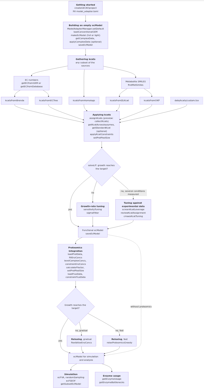
The workflow overview shows the order of the stages, the kcat sources that run in parallel and the alternative paths, with the functions of each stage in MATLAB and Python.

Pages

Start:

• Introduction to ecModels, what an ecModel is and how GECKO adds enzyme constraints to a conventional GEM.

• Installation, set up GECKO or geckopy.

Steps, in the order of the work:

1. Getting started, scaffold a project and fill the model adapter.

2. Building an empty ecModel, expand a conventional GEM into the structure of an ecModel.

3. Gathering kcats, collect the kcats of each source.

4. Applying kcats, write kcats into the enzyme constraints of the ecModel.

5. Growth-rate tuning, close the gap between the growth rate of a new ecModel and that of the organism.

6. Tuning against experimental data, fit and curate the kcats that limit the model.

7. Proteomics integration, constrain the concentrations of individual enzymes with proteomics data.

8. Relaxing overconstrained proteomics, loosen proteomics constraints that keep the ecModel from its growth rate.

9. Simulation and analysis, objectives, flux variability, sampling, flux scanning, mapping to the conventional GEM and context-specific ecModels.

10. Enzyme usage and bottlenecks, which enzymes a solution uses and which enzymes limit the objective.

Background, the reference material that the steps link to:

• GECKO light and full ecModels, the two ecModel layouts and the choice between them.

• ecModel YAML format, the file format that both toolboxes read and write.

• Files in the data folder, every file that the data folder of a project can hold.

• Model adapter parameters, every parameter of model_adapter.toml in both languages.

• Basic model operations, bounds, objectives, FBA, flux inspection and export for conventional GEMs and ecModels.

Migration, pages for GECKO 3 projects and scripts:

• GECKO 3 to GECKO 4, the changes of results, errors, functions and names.

• Project format 4, the project folder, model_adapter.toml, kcat source files and the ecModel format.

• Upgrade a GECKO 3 project, the steps of upgradeGECKOproject and upgradeEcModel.

• Kcat assignment, the kcat sources, stages and presets of collectKcats and assignKcats.

Approximate timing

The table lists the wall-clock time of a first pass through each step on a genome-scale model such as yeast-GEM. The time depends on the size of the model, the internet connection and the configured solver.

Pages	Approximate time	Notes
Getting started, Building an empty ecModel	15 min
Gathering kcats, Applying kcats	1 h	the prediction of kcats accounts for most of the time
Growth-rate tuning, Tuning against experimental data	15 min
Proteomics integration	15 min
Relaxing overconstrained proteomics	15 min	longer with proteomics data of lower quality, which needs more enzymes to be flexibilised
Simulation and analysis	3 h	ecFVA at genome scale accounts for most of the time, and it is much shorter with a commercial solver
Enzyme usage and bottlenecks	15 min

See also

• GECKO 3 to GECKO 4, the changes of GECKO 4 against the published protocol.

• API reference, the generated documentation of the functions of both toolboxes.

• MATLAB vs Python, the names of the functions in GECKO and geckopy.